PythonによるLeNetネットワークモデルの学習と予測

2022-01-02 20:07:45

1. LeNetモデル学習スクリプト

全体の学習コードは以下の通りですが、以下、コードの意味を詳しく説明します。

import torch
import torchvision
from torchvision.transforms import transforms
import torch.nn as nn
from torch.utils.data import DataLoader
from pytorch.lenet.model import LeNet
import torch.optim as optim
import numpy as np
import matplotlib.pyplot as plt

transform = transforms.Compose(
    # Convert the dataset into tensor form
    [transforms.ToTensor(),
     # Normalize, 0.5 is the mean and the variance, corresponding to 0.5 for all three dimensions
     normalize((0.5, 0.5, 0.5), (0.5, 0.5, 0.5))]
)

# When downloading the complete dataset, download=True, the first one is the path to save, after downloading, download should be changed to False
# train=True for the training set, train=False for the test set
train_set = torchvision.datasets.CIFAR10('. /data', train=True,
                                         download=False, transform=transform)

# load training set, set batch size, whether to mess up, number_works is the number of threads, window not set to 0 will report an error, linux can set non-zero
train_loader = DataLoader(train_set, batch_size=36,
                          shuffle=True, num_workers=0)

test_set = torchvision.datasets.CIFAR10('. /data', train=False,
                                        download=False, transform=transform)
# Set batch size to pass in all test set images at once
test_loader = DataLoader(test_set, batch_size=10000,
                         shuffle=False, num_workers=0)

# Iterate over the test set image data and label values
test_img, test_label = next(iter(test_loader))

# Ten class names for CIFAR10
classes = ('plane', 'car', 'bird', 'cat', 'deer',
           'dog', 'frog', 'horse', 'ship', 'truck')

# ---------------------------- shows the image -----------------------------------
# def imshow(img, label):
# fig = plt.figure()
# for i in range(len(img)):
# ax = fig.add_subplot(1, len(img), i+1)
# nping = img[i].numpy().transpose([1, 2, 0])
# npimg = (nping * 2 + 0.5)
# plt.imshow(npimg)
# title = '{}'.format(classes[label[i]])
# ax.set_title(title)
# plt.axis('off')
# plt.show()
# plt.show() 
# 
# batch_image = test_img[: 5]
# label_img = test_label[: 5]
# imshow(batch_image, label_img)
# # ----------------------------------------------------------------------

net = LeNet()
# Define the loss function, nn.CrossEntropyLoss() comes with a softmax function, so the last layer of the model does not need softmax for activation
loss_function = nn.CrossEntropyLoss()
# Define the optimizer, which optimizes all parameters of the network model
optimizer = optim.Adam(net.parameters(), lr=0.001)

# iterate five times
for epoch in range(5):
    # Initial loss is set to 0
    running_loss = 0
    # Loop through the training set, starting from 1
    for step, data in enumerate(train_loader, start=1):
        inputs, labels = data
        # zero_gradient of the optimizer, each loop needs to be zeroed, otherwise the gradients will be stacked infinitely, which is equivalent to increasing the batch size
        optimizer.zero_grad()
        # Input the image data into the model
        outputs = net(inputs)
        # Pass in the predicted and true values, and calculate the current loss value
        loss = loss_function(outputs, labels)
        # Backward propagation of loss
        loss.backward()
        # Perform gradient update
        optimizer.step()
        # Calculate the total loss for the round, since loss is a tensor type, you need to use item() to get the exact value
        running_loss += loss.item()
        # Print the log every 500 times to make a prediction on the test set
        if step % 500 == 0:
            # torch.no_grad() is context management, no gradient updates for testing, no gradient tracking
            with torch.no_grad():
                # Pass in all test set images for prediction
                outputs = net(test_img)
                # torch.max() in dim=1 because the result is in the form of (batch, 10), we only need to take the maximum of the second dimension
                # max this function returns [max, max index], we just need to take the index on the line, so use [1]
                predict_y = torch.max(outputs, dim=1)[1]
                # (predict_y == test_label) the same return True, not equal return False, sum() on the correct rate of superposition
                # Because the variables calculated are tensor, so you need to use item() to get the value
                accuracy = (predict_y == test_label).sum().item() / test_label.size(0)
                # running_loss/500 is to calculate the loss for each step, i.e. the loss for each step
                print('[%d, %5d] train_loss: %.3f test_accuracy: %.3f' %
                      (epoch+1, step, running_loss/500, accuracy))
                running_loss = 0.0

print('Finished Training!')

save_path = 'lenet.pth'
# Save the model, in dictionary form
torch.save(net.state_dict(), save_path)

(1). CIFAR10データセットのダウンロード

ここではtorchvision.datasetが提供するCIFAR10データセットを使用します（その他のデータセットはpytorchのウェブサイトにあります）。 pytorchのウェブサイトから提供されたデータセット )

train_set = torchvision.datasets.CIFAR10('. /data', train=True,
                                         download=False, transform=transform)
test_set = torchvision.datasets.CIFAR10('. /data', train=False,
                                        download=False, transform=transform)

この部分はCIFAR10をダウンロードするためのコードで，最初のパラメータはダウンロードしたデータセットへのパス，train=TrueとFalseはダウンロードしたトレーニングセットとテストセットに対応，transformは対応する画像強調方法です．

(2). 画像補正

transform = transforms.Compose(
    # Convert the dataset into tensor form
    [transforms.ToTensor(),
     # Normalize, 0.5 is the mean and the variance, corresponding to 0.5 in all three dimensions
     normalize((0.5, 0.5, 0.5), (0.5, 0.5, 0.5))]
)

これは、単純な画像イメージの向上、transforms.ToTensor（）は、テンソルにデータセットのすべての画像になり、transforms.Normalize（）は、平均値と標準偏差に対応する2つのタプルを含む正規化処理、各タプルは画像の3次元（チャンネル、高さ、幅）、なぜこれがソートされて、尋ねない、尋ねるpytorch要件であり、順序が変化することはありません、その後に変換を表示されます。正規化（[0.485、0.406、0.456]、[0.229、0.224、0.225]）データのこれらの二つのグループは、これは公式の平均値と標準偏差は、しばしばその後、正規化時に使用されますです。

(3). データセットを読み込む

# load the training set, set the batch size, whether to mess up, number_works is the number of threads, window will report an error if not set to 0, linux can set non-zero
train_loader = DataLoader(dataset=train_set, batch_size=36,
                          shuffle=True, num_workers=0)
test_loader = DataLoader(dataset=test_set, batch_size=36,
                         shuffle=False, num_workers=0)

最初に読み込むのはトレーニングセットとテストセット、shuffle=Trueはデータセットが破壊されること、batch_sizeは36枚の写真を一度にデバイスに入れ、バッチにパックすること、そして写真の形状は[3, 32, 32]----" になることです。[36、3、32、32]は、ネットワークモデルに渡された形状も[なし、チャンネル、高さ、幅]でなければなりません、なしは、バッチの写真の数を表し、それ以外の場合は、エラーを報告する、番号_作品は、スレッドの数、ウィンドウシステムは、エラーを報告する、Linuxシステムは0以外の番号に設定することができる0に設定する必要があります。

(4). 画像の一部を表示する

def imshow(img, label):
    fig = plt.figure()
    for i in range(len(img)):
        ax = fig.add_subplot(1, len(img), i+1)
        nping = img[i].numpy().transpose([1, 2, 0])
        npimg = (nping * 2 + 0.5)
        plt.imshow(npimg)
        title = '{}'.format(classes[label[i]])
        ax.set_title(title)
        plt.axis('off')
    plt.show()


batch_image = test_img[: 5]
label_img = test_label[: 5]
imshow(batch_image, label_img)

この部分は、テストセットの最初の5枚の画像を表示するためのもので、実行後、5枚のスティッチされた画像を表示します

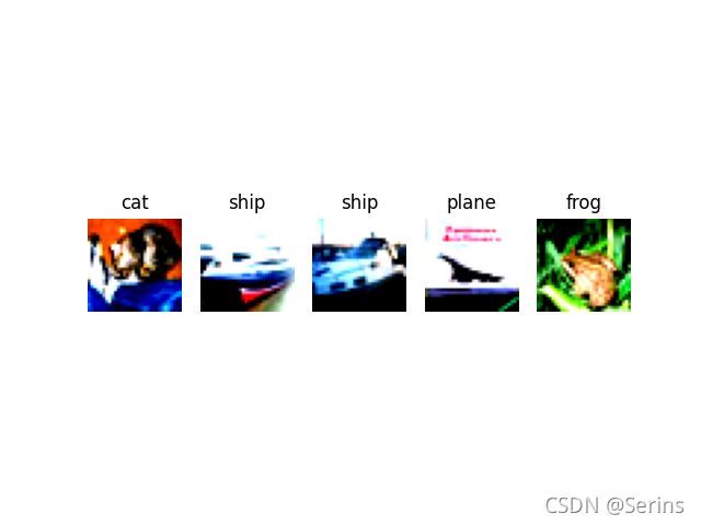
このデータセットの写真は比較的小さいので、32x32のサイズで、いくつかはまた、あまりにも明確に表示されないかもしれませんが、表示された画像は、実際のラベルです、注：画像を表示するコードは、このアラーム（RGBデータでimshowの有効範囲に入力データをクリッピング（フロートの[0 ...1]、整数で [0...255] ）かもしれない。）この警告の解決策としては、画像配列をuint8型に変換する、つまり、plt.imshow(npimg.astype('uint8')とすればよいのですが、そうすると表示画像が変わってしまうので、とりあえずは無視してよいでしょう。

(5). モデルの初期化

データ画像を処理した上で、正式な学習プロセスを以下に示します。

net = LeNet()
# Define the loss function, nn.CrossEntropyLoss() comes with a softmax function, so the last layer of the model does not need softmax for activation
loss_function = nn.CrossEntropyLoss()
# Define the optimizer, which optimizes all parameters of the model
optimizer = optim.Adam(net.parameters(), lr=0.001)

最初のLeNetネットワークを初期化し、クロスエントロピー損失関数、およびアダムオプティマイザを定義し、注釈について書かれた、我々はCrossEntropyLoss（）、CrossEntropyLossクラスに有効に表示するには、Ctrl +左マウスボタンすることができますこの標準では、注釈を見ることができますLogSoftmax関数が含まれているので、最終層のLetNetモデルを構築ソフトマックス活性化関数を使用しないように

(6). モデルを学習させ、モデルパラメータを保存する

for epoch in range(5):
    # Initial loss set to 0
    running_loss = 0
    # Loop through the training set, starting at 1
    for step, data in enumerate(train_loader, start=1):
        inputs, labels = data
        # zero_gradient of the optimizer, each loop needs to be zeroed, otherwise the gradients will be stacked infinitely, which is equivalent to increasing the batch size
        optimizer.zero_grad()
        # Input the image data into the model to get the output
        outputs = net(inputs)
        # Pass in the predicted and true values, and calculate the current loss value
        loss = loss_function(outputs, labels)
        # Loss back propagation
        loss.backward()
        # Perform gradient update (update W,b)
        optimizer.step()
        # Calculate the total loss for the round, since loss is a tensor type, you need to use item() to get the value
        running_loss += loss.item()
        # Print the log every 500 times to test the test set
        if step % 500 == 0:
            # torch.no_grad() is context management, no gradient updates for testing, no gradient tracking
            with torch.no_grad():
                # Pass in all test set images for prediction
                outputs = net(test_img)
                # torch.max() in dim=1 because the result is of the form (batch, 10), we only need to take the maximum of the second dimension, the second dimension is a vector containing the probability of each of the ten categories
                # max this function returns [max, max index], we only need to take the index on the line, so use [1]
                predict_y = torch.max(outputs, dim=1)[1]
                # (predict_y == test_label) the same return True, not equal return False, sum () on the correct results of the superposition, and finally divided by the total number of test set labels
                # Because the calculated variables are tensor, so you need to use item() to get the value
                accuracy = (predict_y == test_label).sum().item() / test_label.size(0)
                # running_loss/500 is to calculate the loss for each step, i.e. the loss for each step
                print('[%d, %5d] train_loss: %.3f test_accuracy: %.3f' %
                      (epoch+1, step, running_loss/500, accuracy))
                running_loss = 0.0
                
print('Finished Training!')

save_path = 'lenet.pth'
# Save the model, in dictionary form
torch.save(net.state_dict(), save_path)

このコードのコメントは非常に明確に書かれている、あなたはプロセスが複雑ではない理解するために注意深く読むことができ、理解するために多くの時間を読んで、最終的に良い（*￣▽￣）に学習したモデルを保存する

2.予測スクリプト

モデルは上記で学習済みで、lenet.pthのパラメータファイルも取得済みなので、予測は非常に簡単です。

import torch
import numpy as np
import torchvision.transforms as transforms
from PIL import Image
from pytorch.lenet.model import LeNet

classes = ('plane', 'car', 'bird', 'cat', 'deer',
           'dog', 'frog', 'horse', 'ship', 'truck')

transforms = transforms.Compose(
    # Resize the data image
    [transforms.Resize([32, 32]),
     ToTensor(),
     Normalize((0.5, 0.5, 0.5), (0.5, 0.5, 0.5))]
)

net = LeNet()
# Load the pre-trained model
net.load_state_dict(torch.load('lenet.pth'))
# A random image of a cat found online
img_path = '... /... /Photo/cat2.jpg'
img = Image.open(img_path)
# Image processing
img = transforms(img)
# Add a dimension, (channels, height, width)------->(batch, channels, height, width), pytorch requires such a shape to be entered
img = torch.unsqueeze(img, dim=0)

with torch.no_grad():
    output = net(img)
    # dim=1, take only the dimension of the 10 categories in [batch, 10], take the maximum index of the prediction, and convert to numpy type
    prediction1 = torch.max(output, dim=1)[1].data.numpy()
    # Use softmax() to predict a probability matrix
    prediction2 = torch.softmax(output, dim=1)
    # Get the index of values with the highest probability
    prediction2 = np.argmax(prediction2)
# Both ways to get the final result
print(classes[int(prediction1)])
print(classes[int(prediction2)])

とにかく、私は猫が犬であることを識別するために結果を予測し、90.01％の確率で、とんでもないハハッに終わったが、またLeNetはネットワークモデルが本当に浅いことを示し、特徴抽出は、これが発生するのに十分深くないです。

PythonによるLeNetネットワークモデルの学習と予測に関する記事は以上です。LeNetネットワークモデルの学習と予測については、BinaryDevelopの過去の記事を検索するか、以下の記事を引き続き閲覧してください。