[CSSチュートリアル】波動効果を生み出すCSSのアイデア
前回、純粋なCSSを使って波動効果を実装する方法をいくつか紹介しましたが、それについて関連する記事が2つあります。
今回は、CSSを使った波動効果の面白いアイデアをもう一つ取り上げます。
曲がった三角形の面積の定積分から始める
本題に入る前に、これを見てください。高等数学では、二次曲線グラフの面積を定積分で求めることができます。
曲線の下の領域を細かい高さのn個の長方形に分割し、nが無限大になるにつれて、すべての長方形の面積が曲線のグラフの面積に等しくなるようにすればよいのです。
から引用した2つの簡単な模式図。 なぜ定積分は面積を求めることができるのか? :
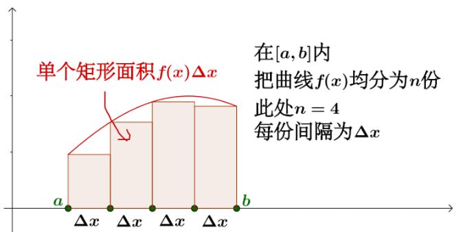
nが無限大に近づくと、すべての長方形の面積は、曲面グラフの面積と等しくなるとき。
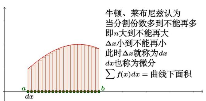
このアイデアを使えば、CSSでも複数のdivで曲線のエッジ、つまり波線をシミュレートすることができる。
ステップ1.グラフィックを複数枚に切り分ける
まず、親コンテナを定義し、その下に12個の子 div を定義します。
"""


import numpy as np


from scipy.optimize import leastsq


def func(x, p):


"""
By
"""


A, k, theta = p


return A*np.sin(2*np.pi*k*x+theta)
def residuals(p, y, x):


"""
レイアウト、シンプルなレイアウトでは、このように各子要素の高さが等しいグラフが得られます。
"""


return y - func(x, p)


x = np.linspace(-2*np.pi, 0, 100)


A, k, theta = 10, 0.34, np.pi/6 # function arguments for real data


y0 = func(x, [A, k, theta]) # real data


# Experimental data after adding noise


y1 = y0 + 2 * np.random.randn(len(x))


p0 = [7, 0.2, 0] # First-guess function fit parameters
# call leastsq to fit the data, residuals is the function that calculates the error


# p0 is the initial value of the fit parameters, # args is the experimental data to be fitted


plsq = leastsq(residuals, p0, args=(y1, x))


# In addition to the initial values, the args argument is called to specify the other parameters used in the residuals (the global variables for x,y are used directly in the linear fit), again returning a tuple with the first element being the array of parameters after the fit.
Here (y1, x) is passed to the args argument. leastsq() will pass these two additional arguments to residuals(). Thus residuals() has three arguments, p for the sine function, and y and x for the array representing the experimental data.


print u"Real Parameters:", [A, k, theta]


print u "Fitted parameters", plsq[0] # Parameters after fitting to experimental data


import pylab as pl


pl.plot(x, y0, label=u"real data")


pl.plot(x, y1, label=u"Experimental data with noise")


pl.plot(x, func(x, plsq[0]), label=u"Fitted data")


pl.legend()


pl.show()
>>> Real Parameters: [10, 0.340000000000000000002, 0.52359877559829882]


>>> Fitted parameters [-9.84152775 0.33829767 -2.68899335]
その効果は次の通りです。
ステップ2. 各子要素に、異なる負の遅延で高さ変換アニメーションを実行させる
次に、簡単な模様替えをするために、グラフを動かす必要がありますが、これは、各子要素の高さを
minimize(fun, x0[, args, method, jac, hess, ...]) Minimization of scalar function of one or more variables.
Note: The parameter bounds=((0,None), (0,None)) represents the bounds corresponding to each dimension of x. If there is only one dimension, write bounds= ((0, None), ) as well, or use the following minimize_scalar function.
bounds= ((0, None), (0, None)) corresponds to the initial value x0 of x, which should be two-dimensional, as in (1, 0).
For example see [
scipy.optimize.minimize
]


 minimize_scalar(fun[, bracket, bounds, ...]) Minimization of scalar function of one variable.
Note: These functions, such as minimize_scalar, return an OptimizeResult object, and print() results like this.
 fun: -2.3627208257312922


    nfev: 9


     nit: 8


 success: True


       x: 1.333333333395553
その効果は次の通りです。
次に、各子要素のアニメーションシーケンスに、異なる時間の負の遅延を設定させるだけで、予備的な波の効果が得られますが、ここでは作業負荷を軽減するためにSASSの助けを借りて実装しています。
def test():
    import math
    from scipy import optimize
    func = lambda x: x * math.log(x, 2)
    a = optimize.optimize_scalar(func, bounds=[0.1, 1], method='bounded')
    print(a)
これによって、予備的な波動効果である
ステップ3.ジャギーをなくす
上の波のアニメーションはご覧の通り、ジャギーが出ているので、できるだけジャギーをなくすようにします。
方法1:divの数を増やす
冒頭の曲線グラフの面積を定積分で求める考え方にならい、子divの数をできるだけ増やせばよく、divの数が無限になれば、ジャギーは消えます。
上の12個のサブディビジョンを120個に置き換えてみることができます。120個のdivをひとつひとつ書くのは面倒なので、ここでは パグ テンプレートエンジン
     fun: -0.5307378454230427


 message: 'Solution found.'


    nfev: 9


  status: 0


 success: True


       x: 0.3678794534141907
関連
-
[CSSチュートリアル】背景-位置の割合の原則の説明
-
[CSSチュートリアル】CSSの新機能には、ページの再描画や並び替えの問題をコントロールする機能が含まれています。
-
[CSSチュートリアル】CSSカウンターを使った数字の並びの美化方法
-
[CSSチュートリアル】擬似要素で実現する中空三角矢印とXアイコンの例
-
[CSSチュートリアル】空間均等性の問題を解決する2つの方法
-
[CSSチュートリアル]テーブル table :nth-child()を使って行間の色変更と整列を実現する。
-
[CSSチュートリアル】CSS複合セレクタの具体的な使用方法
-
[CSSチュートリアル】大きな画像や情報を小さなドロップダウンで実現するCSS
-
[CSSチュートリアル]cssに0.5pxの行を実装してモバイル互換の問題を解決する(推奨)
-
[CSSチュートリアル】CSS擬似クラス:empty makes my eyes shine(コード例)
最新
-
nginxです。[emerg] 0.0.0.0:80 への bind() に失敗しました (98: アドレスは既に使用中です)
-
htmlページでギリシャ文字を使うには
-
ピュアhtml+cssでの要素読み込み効果
-
純粋なhtml + cssで五輪を実現するサンプルコード
-
ナビゲーションバー・ドロップダウンメニューのHTML+CSSサンプルコード
-
タイピング効果を実現するピュアhtml+css
-
htmlの選択ボックスのプレースホルダー作成に関する質問
-
html css3 伸縮しない 画像表示効果
-
トップナビゲーションバーメニュー作成用HTML+CSS
-
html+css 実装 サイバーパンク風ボタン
おすすめ
-
[CSSチュートリアル】CSS たった1行のコードでアバターと国旗の一体化を実現
-
[CSS3] CSS3リスト無限スクロール/回転効果
-
[CSSチュートリアル]cssの位置固定コードで左右2重の位置決め
-
[CSSチュートリアル】CSSもこんな風に遊べる?気まぐれグラデーションの極意
-
[CSSチュートリアル】CSSで実現するTikTokのテキストジッター効果例
-
[css3]Webコードのグレーまたはブラックモードを実現するCSS3フィルター(filter)
-
[CSSチュートリアル】cssプロパティ width デフォルト値 width: auto と width: 100% の違いを解説。
-
[CSSチュートリアル]css use negative margin to achieve average layout of example.
-
[CSSチュートリアル】CSSのラインハイトとハイトを詳しく解説
-
[css3]CSS3トランジションによる通知メッセージ回転バーの実装